Quick Start

IQM Pulla is a client-side Python package which allows the user to control the generation and execution of pulse-level instruction schedules on a quantum computer. Within the existing IQM QCCSW stack, Pulla is somewhere between circuit-level execution and dedicated calibration experiments. Namely, with pulse-level access the user can:

• compile a quantum circuit (e.g. from Qiskit) into an instruction schedule on the client side

• access and modify the calibration data to be used for the circuit-to-schedule compilation

• view and modify the default implementations of quantum gates, using e.g. custom pulse shapes

• define custom implementations of quantum gates

• define new composite gates out of native gates and set their calibration data

• control the multi-step compilation procedure, and edit the intermediate data

• construct instruction schedules manually

This notebook contains a small meaningful example for a “quick start”. Refer to other chapters for more details on various aspects of Pulla.

Authentication

The preferred way to provide the connection and authentication information to Pulla is using environment variables.

• Pulla (and IQMClient) connect to the quantum computer using the URL in the environment variable IQM_SERVER_URL.

• IQM Server uses bearer token authentication to manage access to quantum computers. Get your personal token from the IQM Server web dashboard and store it in the environment variable IQM_TOKEN, where Pulla (and IQMClient) will find it.

• For IQM Server instances that manage more than one quantum computer you need to also provide the name of the quantum computer in the environment variable IQM_QUANTUM_COMPUTER.

Alternatively, the connection and authentication information can be provided explicitly to Pulla.__init__,

p = Pulla("<IQM Server URL>", quantum_computer="<quantum computer name>", token="<your API token>")

or the environment variables can be set inside the notebook using

import os
os.environ["IQM_SERVER_URL"] = "<IQM Server URL>"
os.environ["IQM_QUANTUM_COMPUTER"] = "<quantum computer name>"
os.environ["IQM_TOKEN"] = "<your API token>"

However, this is not recommended since this way it is easy to accidentally expose your API token e.g. when giving a presentation or by committing the notebook with the API token to a shared code repository.

Using Pulla with IQM Resonance

Pulla can also be used with the IQM Resonance cloud service. You need to set IQM_SERVER_URL to point to Resonance (https://resonance.iqm.tech), and specify the quantum computer to use in IQM_QUANTUM_COMPUTER.

The names of the available quantum computers can be found on the Resonance dashboard.

from qiskit import QuantumCircuit, visualization
from qiskit.compiler import transpile
from iqm.iqm_client.util import print_env_vars
from iqm.qiskit_iqm import IQMProvider
from iqm.pulla.pulla import Pulla
from iqm.pulla.utils_qiskit import qiskit_to_pulla, sweep_job_to_qiskit

print_env_vars()

# Create a Pulla client and a qiskit-iqm backend for accessing the quantum computer.
p = Pulla()
provider = IQMProvider()
backend = provider.get_backend()

# Define a quantum circuit.
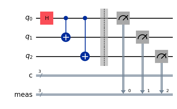
qc = QuantumCircuit(3, 3)
qc.h(0)
qc.cx(0, 1)
qc.cx(0, 2)
qc.measure_all()

qc.draw(output='mpl')

# Transpile the circuit using Qiskit
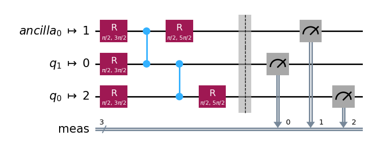
qc_transpiled = transpile(qc, backend=backend, layout_method='sabre', optimization_level=3)
qc_transpiled.draw(output="mpl")

# Convert it into Pulla format
circuits, compiler = qiskit_to_pulla(p, backend, qc_transpiled)

# Set the number of shots
shots = 100
settings = compiler.get_settings(circuits=circuits)
settings.set_shots(shots)

# Compile the circuit into a job definition containing a playlist of instruction schedules.
job_definition, context = compiler.compile(circuits, settings=settings)

# Pulla.submit_playlist() returns an object that tracks the state of the job on the server.
# The measurements are obtained using job.result() after job.wait_for_completion().
job = p.submit_playlist(job_definition, context=context)
job.wait_for_completion()
qiskit_result = sweep_job_to_qiskit(job, shots=shots)

print(f"Raw results:\n{job.result().circuit_measurement_results}\n")
print(f"Qiskit result counts:\n{qiskit_result.get_counts()}\n")
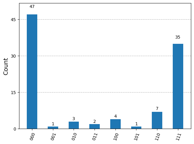
visualization.plot_histogram(qiskit_result.get_counts())

[06-08 15:22:35;I] Waiting for job 019ea72f-4c3d-7640-a38a-a4ffa05a1411 to finish...

Raw results:
[{'meas_3_1_0': [[0], [0], [0], [1], [0], [1], [1], [0], [0], [0], [0], [0], [0], [0], [1], [1], [0], [1], [0], [0], [0], [0], [0], [1], [0], [0], [0], [0], [1], [0], [1], [0], [0], [0], [1], [0], [0], [0], [1], [1], [1], [0], [1], [1], [0], [0], [1], [0], [0], [0], [1], [1], [0], [1], [1], [1], [0], [0], [0], [1], [1], [0], [0], [0], [0], [0], [0], [0], [1], [1], [0], [0], [1], [0], [1], [0], [0], [0], [1], [1], [1], [0], [1], [1], [0], [0], [1], [1], [0], [1], [0], [1], [0], [0], [0], [1], [1], [0], [0], [1]], 'meas_3_1_1': [[0], [0], [0], [1], [0], [1], [1], [0], [0], [0], [0], [0], [0], [1], [1], [1], [0], [1], [0], [1], [1], [0], [0], [1], [0], [1], [1], [0], [1], [0], [1], [0], [0], [1], [1], [0], [1], [0], [1], [1], [1], [0], [1], [1], [0], [0], [0], [0], [0], [0], [1], [1], [0], [1], [1], [1], [0], [0], [0], [1], [1], [0], [0], [0], [0], [0], [0], [1], [1], [1], [0], [0], [1], [0], [1], [0], [0], [0], [1], [1], [1], [1], [1], [0], [0], [1], [1], [1], [0], [1], [0], [1], [0], [0], [0], [1], [1], [0], [0], [1]], 'meas_3_1_2': [[0], [0], [0], [1], [0], [1], [1], [0], [0], [0], [0], [0], [0], [1], [0], [1], [0], [1], [0], [1], [1], [0], [0], [1], [0], [0], [0], [0], [1], [0], [1], [0], [0], [1], [1], [0], [1], [0], [1], [1], [1], [0], [1], [1], [0], [0], [0], [0], [0], [0], [1], [1], [0], [1], [1], [1], [0], [1], [1], [1], [1], [0], [0], [0], [0], [0], [0], [0], [1], [1], [0], [0], [0], [0], [1], [0], [0], [1], [1], [1], [1], [1], [1], [1], [0], [1], [1], [1], [0], [1], [1], [1], [0], [0], [0], [1], [1], [0], [0], [1]]}]

Qiskit result counts:
{'000': 47, '111': 35, '110': 7, '011': 2, '010': 3, '001': 1, '100': 4, '101': 1}

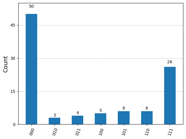
# The results should be comparable to a direct circuit execution through IQM Server.
print("Executing the same circuit via the Qiskit backend...")
job = backend.run(qc_transpiled, shots=shots)
print(f"Qiskit result counts from IQM Server:\n{job.result().get_counts()}")

visualization.plot_histogram(job.result().get_counts())

Executing the same circuit via the Qiskit backend...
[06-08 15:22:39;I] Waiting for job 019ea72f-5c81-73b1-95fc-e5ee5a82b5e0 to finish...
Qiskit result counts from IQM Server:
{'000': 50, '111': 26, '101': 6, '011': 4, '110': 6, '100': 5, '010': 3}

Schedule visualization

IQM Pulse comes with a schedule visualizer. It takes a Playlist (i.e. a compressed list of instruction schedules) and a list of schedule/segment indices to inspect. The playlist variable below is the one which we derived from the original Qiskit circuit using the Pulla compiler, and it only has one schedule.

from iqm.pulse.playlist.visualisation.base import inspect_playlist
from IPython.core.display import HTML

HTML(inspect_playlist(job_definition.sweep_definition.playlist, [0]))